Designing drugs with a quantum computer
With every new hardware architecture comes an accompanying software architecture, and when the two meet, there is a cambrian explosion of invention and innovation. We are experiencing this now with GPUs + transformers.
Driven primarily by curiosity, I wondered what one of the use cases for quantum computers would be. We hear about how they break encryption algorithms, but besides that, there really isn’t anything. So what can you do on a quantum computer that you can’t on a classical computer?
Biotech
Most of my work in the past couple of years has been at the intersection of computers, engineering, information, and biology. When we design a drug, we are designing a smaller molecule that can fit into a larger molecule to turn off the larger molecule or turn on some desired function. At the molecular level, this is how a lot of biology works — stuff is expressed/repressed based on turning it on or off.
Last year, I found this paper where the authors used new computational tools to make antivenom binders to neutralize cobra toxins. The design and filtering process was done completely in silico. They then injected these binders into mice poisoned with cobra venom, and every treated mouse survived.
We could do the same simulation with a quantum computer, but there are too few qubits in the world to simulate a binder docking into a protein. A physicist I met recently that works on applying qubits to chemical models was fundraising to port Boltz2 to quantum, but said we are orders of magnitude away (does not mean it is impossible, just expensive).
All that to say, we can work through a toy example today that can someday compound into fitting a binder into a protein.
What are we actually trying to compute?
Almost everything we care about in a molecule, whether a bond holds, how a reaction proceeds, how tightly a drug sits in a binding pocket; is governed by the energy of its electrons. Formally, the electronic structure problem is an eigenvalue problem:
The quantity that matters most is the ground-state energy, : the smallest eigenvalue of the molecular Hamiltonian . Differences in across geometries give us potential energy surfaces, reaction barriers, and binding affinities.
So the whole game is finding . The rest of this post builds a tiny drug-design stack, one layer at a time. Each layer only works because of the one under it:
| Layer | What it honestly does | Status |
|---|---|---|
| 1. Quantum | Exact energies for small, hard pieces of a molecule, like metal active sites or bonds breaking, where classical approximations get the answer wrong | Toy-sized today. Useful once qubits are error-corrected |
| 2. Machine learning | Learns from those exact energies, then scales up to protein size. “Nearsightedness” is what makes that work | Works today with classical training data |
| 3. Swarm agents | Split the molecule into fragments. Each agent owns one fragment on its own small set of qubits, and a coordinator stitches the answers together | Easy to run in parallel on simulators today |
| 4. Binder-pocket fitting | Binding energy = E(complex) − E(pocket) − E(ligand). The quantum part only handles the core of the pocket | Classical tools like Boltz-2 and BindCraft still win |
| 5. Quantum signals from the body | Quantum sensors: diamond magnetometers, wearable brain scanners (OPM-MEG), hyperpolarized MRI | Already in use. Probably the most real quantum-in-biology story right now |
| 6. Generative design | Quantum circuits as the random-sampling part of a molecule generator | Early, and whether it beats classical methods is disputed |
Every experiment below runs on a laptop in a few minutes, except the part that runs on a real quantum computer. The molecules are as small as molecules get: hydrogen. That’s on purpose. Hydrogen is the “hello world” of quantum chemistry, and every idea here scales up to drug-sized problems in principle. In practice, that’s the part that costs a few more decades and a few million more qubits.
1. Quantum: the energy calculator
Builds on: above.
To put H₂ on a quantum computer, you describe each electron’s possible orbitals with a small set of basis functions. Hydrogen in the smallest basis has 2 spatial orbitals, each of which can hold a spin-up and a spin-down electron. That’s 4 slots, and each slot becomes one qubit: 1 if an electron is there, 0 if not. So H₂ is a 4-qubit problem.
Why bother with qubits at all? Because the classical bookkeeping explodes. 4 qubits hold 2⁴ = 16 amplitudes, which my laptop handles fine. 50 qubits hold about 10¹⁵. A few hundred qubits hold more amplitudes than there are atoms in the universe. A quantum computer doesn’t write those numbers down; the qubits just are that state. That’s the one thing it does that a GPU can’t.
The algorithm is a variational quantum eigensolver (VQE). It’s a loop. The quantum computer prepares a guess for the electrons’ state using a circuit with a few adjustable angles, then measures its energy. A normal classical optimizer nudges the angles and asks again, until the energy stops going down. Since is the smallest eigenvalue, the lowest energy you can find is your best answer.
H, n_qubits = qml.qchem.molecular_hamiltonian(molecule)   # the H in H|ψ⟩ = E|ψ⟩, as qubit operators

@qml.qnode(qml.device("default.qubit", wires=n_qubits))
def energy(angles):
    qml.AllSinglesDoubles(angles, wires=range(n_qubits), hf_state=hf, singles=singles, doubles=doubles)
    return qml.expval(H)                                   # measure ⟨ψ|H|ψ⟩

opt = qml.AdamOptimizer(0.05)
for step in range(400):
    angles, e = opt.step_and_cost(energy, angles)          # classical optimizer, quantum energy
Then I pulled the two hydrogen atoms apart and computed the energy at each distance:
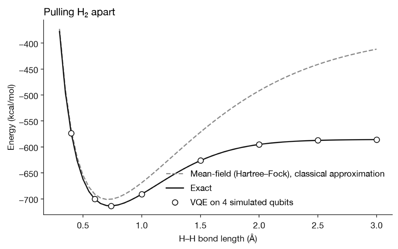
VQE lands on the exact answer at every point, within 0.0003 kcal/mol. The dashed line is Hartree-Fock, the classical “mean-field” approximation, where each electron only feels the average of the others. At the normal bond length it’s off by 13 kcal/mol. Once the bond is stretched to 3 Å it’s off by 174 kcal/mol, because it can’t describe two electrons that each want to go home to a different atom. Breaking bonds, metals and other “strongly correlated” electrons are exactly where classical approximations fail and a quantum computer earns its keep.
On a real quantum computer
Everything above ran on a simulated quantum computer, which is cheating a little. So I ran the same calculation on Rigetti’s 108-qubit Cepheus machine through Amazon Braket: 5 bond lengths, 2,000 shots per circuit, 27 circuits in total, about $31. (A second round, below, cost about $89.)
Two tricks keep the hardware noise down. First, the angle for each bond length is found on the simulator, so the quantum computer only has to measure the energy, not run the whole optimization loop. Second, I rewrote the circuit. The exact H₂ ground state is a mix of just two configurations, both electrons in the bonding orbital or both in the antibonding one, and you can prepare that with one rotation and three CNOT gates instead of the ~14 CNOTs the textbook circuit compiles to. Two-qubit gates are where real hardware makes most of its mistakes, so fewer is better.
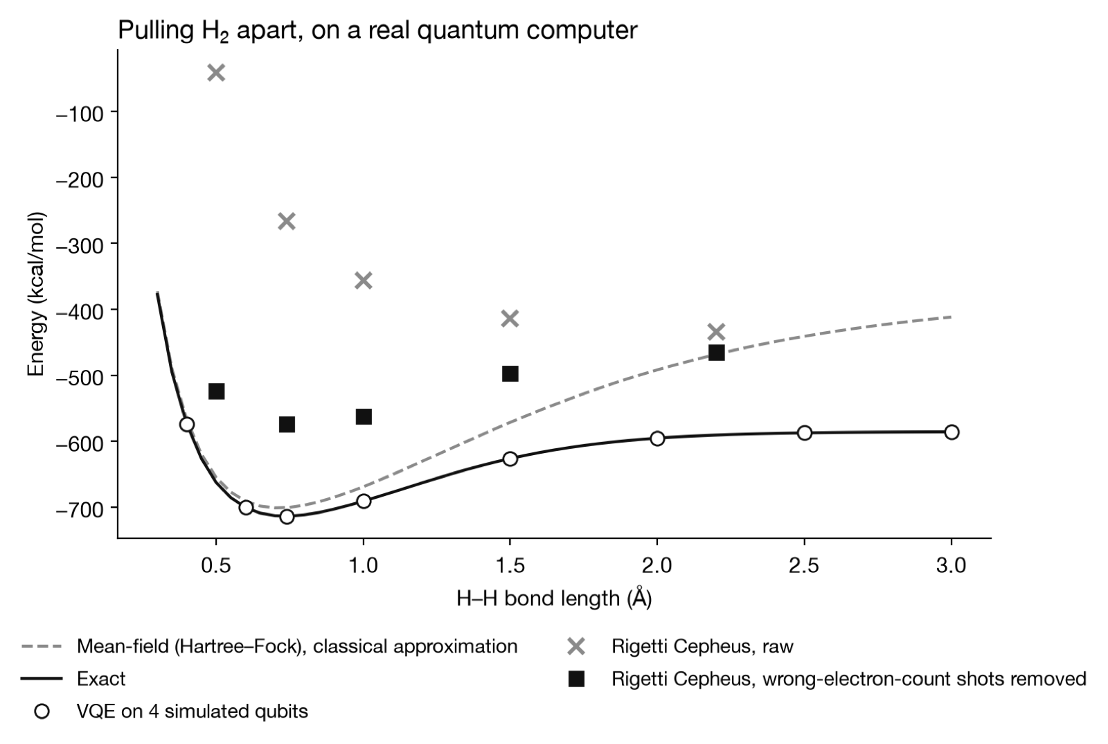
All 27 circuits ran in about two minutes. The results were bad:
| Bond length | Classical mean-field error | Rigetti, raw | Rigetti, bad shots removed | Shots kept |
|---|---|---|---|---|
| 0.50 Å | 8 kcal/mol | 621 | 139 | 30% |
| 0.74 Å | 13 | 448 | 140 | 32% |
| 1.00 Å | 22 | 335 | 128 | 32% |
| 1.50 Å | 55 | 213 | 129 | 37% |
| 2.20 Å | 122 | 157 | 126 | 46% |
At the normal bond length, the real quantum computer was off by 448 kcal/mol. The classical approximation it’s supposed to beat was off by 13.
Rigetti’s compiler wasn’t the problem. I simulated the exact program it compiled and ran: it should produce the right configuration 98.7% of the time. On the hardware, that happened 27% of the time. The most common result had three electrons in a two-electron molecule. When a two-qubit gate fails, it can flip a qubit from “no electron here” to “electron here”, and a state with the wrong number of electrons has a wildly wrong energy.
There’s a standard fix for that specific failure. We know H₂ has exactly two electrons, one spin-up and one spin-down, so any shot that doesn’t is garbage and you can throw it out. That’s called symmetry post-selection. It kept only about a third of the shots, and the error dropped to 126-140 kcal/mol, which is still worse than mean-field at every bond length.
The weird part is the device’s own calibration. It says the three two-qubit gates my circuit used are 99.2-99.5% accurate. Add the read-out errors I measured, and the circuit should land on the right configuration roughly 85% of the time, not 27%. The calibration numbers are measured one gate at a time, in isolation. A real circuit runs gates back to back next to other qubits, and errors (crosstalk, drift since the last calibration) pile up in ways those numbers don’t capture.
So this is where “toy-sized today” comes from. The simulator gets H₂ exactly right, because a simulated qubit doesn’t make mistakes. A real qubit makes so many that a 4-qubit, 3-gate circuit loses to an approximation from the 1930s. Error correction exists to fix exactly this: spend many noisy physical qubits to build one reliable “logical” qubit. Until machines do that at scale, the useful work happens on simulators and in planning for the hardware that’s coming.
Making it less error-prone
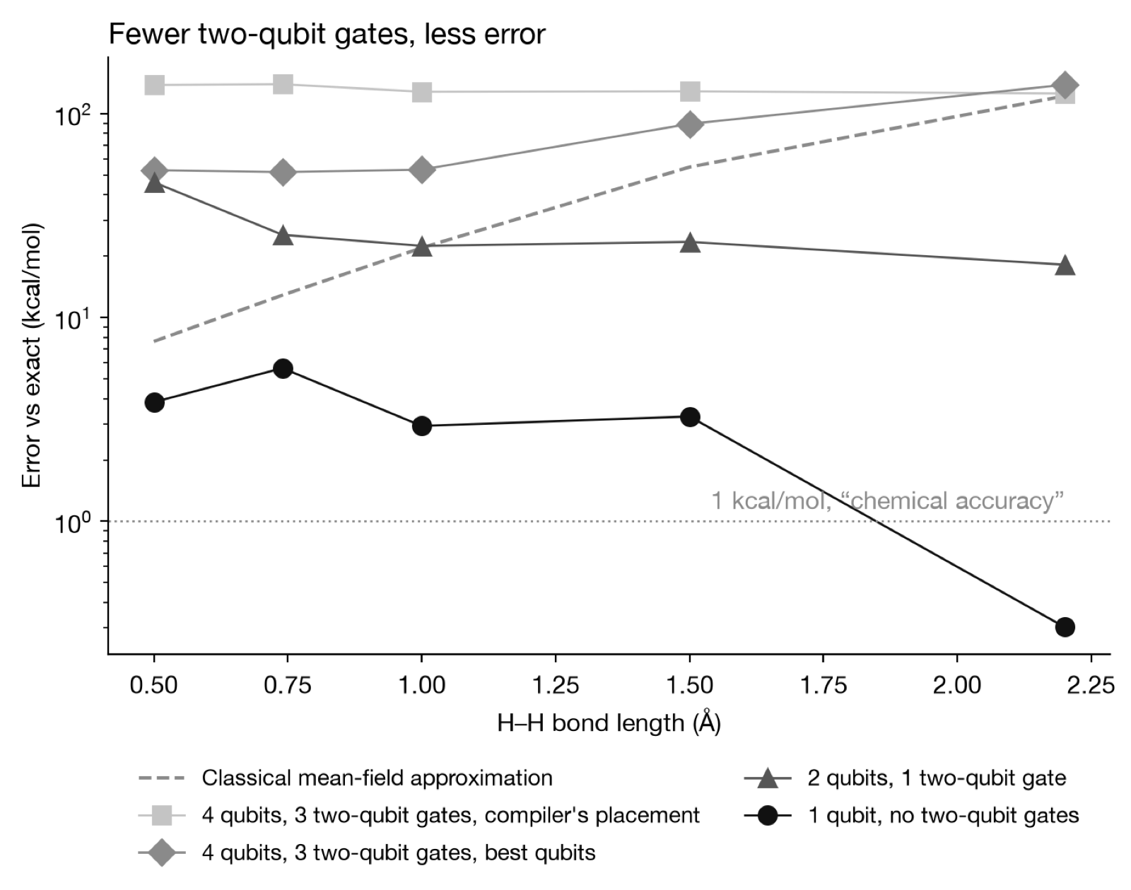
If two-qubit gates are the problem, use fewer of them. I gave myself another $100 and tried three things, all on the same Rigetti machine:
- Shrink the problem to 1 qubit. H₂ has symmetries we already know: two electrons, one spin-up and one spin-down, and so on. Each one fixes the value of one qubit, so you can remove that qubit from the problem entirely. It’s called qubit tapering. H₂ has three of these symmetries, so 4 qubits become 1, and the whole calculation is a single rotation with no two-qubit gates at all.
- Shrink it to 2 qubits. Use two of the three symmetries. That leaves one two-qubit gate, and the leftover symmetry still lets me throw out bad shots.
- Same 4-qubit circuit, better qubits. In the first run, the compiler chose which physical qubits to use. This time I picked them myself from the calibration data: the best-performing qubit on the chip and its three best neighbors.
| Version | Two-qubit gates | Average error | Beats mean-field? |
|---|---|---|---|
| 4 qubits, compiler’s placement | 3 | 132 kcal/mol | No |
| 4 qubits, best qubits | 3 | 77 kcal/mol | No |
| 2 qubits | 1 | 27 kcal/mol | At 1.5 and 2.2 Å |
| 1 qubit | 0 | 3.2 kcal/mol | At every bond length |
Picking good qubits cut the error almost in half, but it wasn’t enough. Every two-qubit gate I removed helped more than anything else I tried. The 1-qubit version beat the classical approximation at every bond length, and at 2.2 Å it landed within chemical accuracy (0.3 kcal/mol). With 4,000 shots, the randomness of measurement alone is worth about 2-3 kcal/mol, so part of that last one is luck.
That’s the honest state of quantum chemistry on hardware today. The real wins come from making the problem fit the machine, not from the machine. Tapering only worked because I already knew H₂’s symmetries. For a drug-sized molecule, the problem doesn’t shrink to one qubit, and you can’t avoid two-qubit gates. That’s why error correction, not more qubits, is the thing to watch.
2. Machine learning: learning from the calculator
Builds on: layer 1’s energies as training labels.
Exact quantum energies are expensive, on a real machine or a simulated one. So you don’t want to ask the quantum computer about every geometry of every molecule. You want to ask it about a few, then train a model to fill in the rest.
So I took 8 VQE energies from the bottom of the H₂ well (0.5 to 1.2 Å) and trained a Gaussian process, a simple ML model that also tells you how unsure it is.
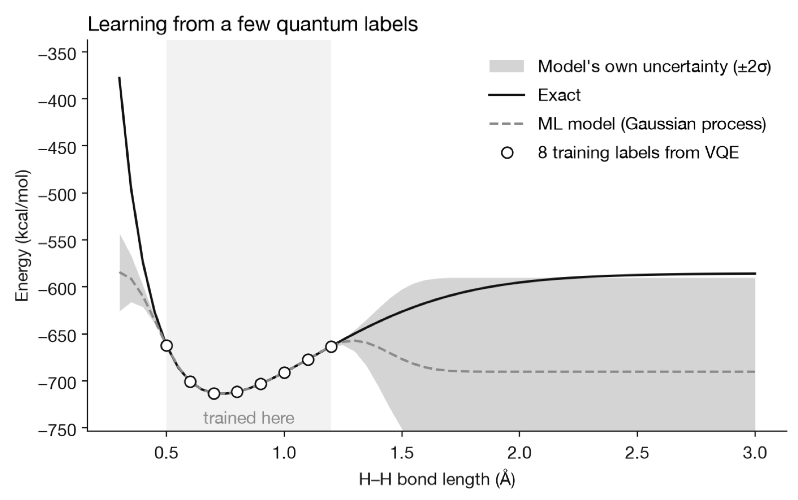
Inside the training range, the model is off by 0.12 kcal/mol on average. Past 1.6 Å it’s off by about 98 kcal/mol. It didn’t see a bond break in training, so it has no idea that one can. To its credit, it knows it doesn’t know: the uncertainty band blows up right where the model goes wrong.
That’s the same problem the people working on ML-accelerated DFT are fighting, at a much bigger scale.
I found this really cool X post where this lab created an algorithm to make density function theory scale linearly with input size. Out of laziness, here is Claude on it:
What DFT is. Density functional theory is the workhorse method for simulating molecules and materials at the quantum level. The exact quantum description of a molecule is a wavefunction that depends on every electron’s position at once, which is hopelessly expensive. DFT’s trick (Hohenberg, Kohn, and Sham, mid-1960s, hence “60-year-old”) is that you don’t need the full wavefunction. The electron density — just a 3D cloud of “how much electron is here” — is enough to determine the energy, forces, and structure. So instead of one monstrous many-electron problem, you solve a set of one-electron problems that each feel an averaged-out field from the density. You solve those, get a new density, rebuild the field, and repeat until it stops changing.
Currently, quantum-mechanical simulations take , where if you want to double the input size (or resolution), it costs 8x! (double, so = 8)
They had it scale quasi-linearly, which wasn’t quite their goal, but still a massive improvement. They have some word slop with *“Using a novel Fourier neural operator variant, we learn the underlying Kohn–Sham equation map to produce physics-informed, self-consistent answers,”*but they basically used some new AI methods and it brought the complexity down to .
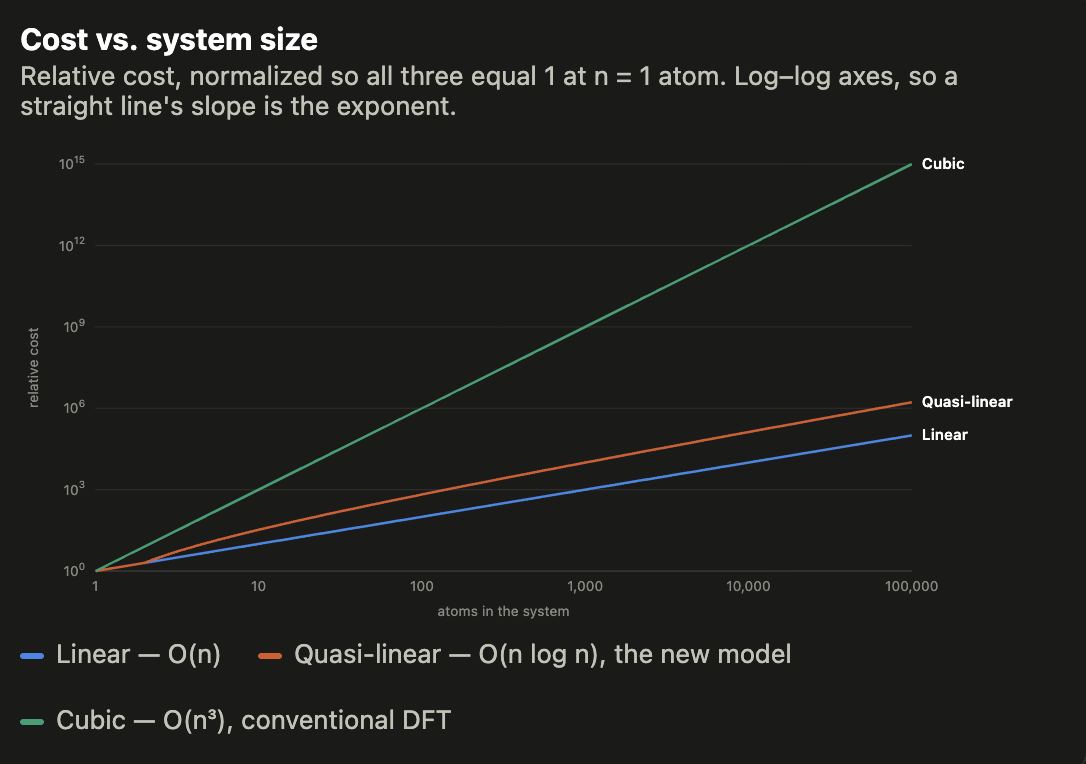
Why is it n³? Those one-electron problems are solved together as one big matrix problem. You describe each electron’s orbital as a combination of some set of basis functions, and the number of basis functions grows in proportion to the number of atoms. Call that N. The physics gets encoded as an NxN matrix (the Hamiltonian), and the core step of each iteration is to diagonalize it — find its eigenvectors, which are the orbitals, and its eigenvalues, which are their energies. Diagonalizing an NxN matrix costs about N³ operations. It’s the same reason inverting a big matrix or multiplying two of them is cubic: for each of N outputs you’re combining N things, each of which involves N terms. Also, to keep all N orbitals orthogonal to each other, you’re comparing every orbital against every other one — N² pairs, each pair costing N to evaluate — cubic again.
Doubling atoms doubles N, and 2³ = 8× the cost. Ten times the atoms is 1,000× the cost, which is why a few hundred atoms is comfortable and tens of thousands is not.
How is it possible that it is not cubic? The cubic cost comes from treating every orbital as spread over the whole system, so everything interacts with everything. But physically, that’s wasteful. An electron on one end of a protein doesn’t care much about atoms 50 Å away; its influence dies off with distance. This is called “nearsightedness,” and it means the true information content of the problem grows only linearly with size. Linear-scaling DFT methods exploit that by working with localized orbitals and throwing away the far-apart interactions. The catch is that doing this well is hard: in metals the nearsightedness is weak, the approximations can wreck accuracy, and the bookkeeping introduces its own overhead. That’s the six-decade struggle.
The AI angle in the tweet is that a learned model can, in effect, absorb the local physics. It can predict what the density or the Hamiltonian looks like around each atom from its neighborhood, so the cost is roughly “number of atoms x cost per neighborhood,” which is linear, plus a log factor from things like neighbor lookups and long-range electrostatics. The hard part the tweet is emphasizing is that such a model has to extrapolate: it’s trained on small systems, because generating quantum-mechanical training data is itself expensive, and it has to remain correct on systems far larger than anything it saw.
So the recipe for the future looks like this: a quantum computer produces a small number of very accurate labels for the hard, local pieces of chemistry, and a nearsighted ML model learns from them and scales to the whole protein. The quantum computer doesn’t see the protein. And the extrapolation problem doesn’t go away, which is why you keep going back to the quantum computer for more labels.
3. Swarm agents: splitting the work
Builds on: layer 2’s nearsightedness. If far-apart atoms barely interact, you can solve them separately.
My first instinct was to spread many agents across many qubits, like threads across CPU cores. That doesn’t work. Qubits aren’t cores. A quantum computer holds one big state across all its qubits, and measuring it collapses that state into a single answer. You can’t read out a thousand parallel answers from one run.
What does work is splitting the molecule. Give each agent one fragment and its own small set of qubits, let them all run at the same time, and have a coordinator add up the answers. Real versions of this exist (fragment methods like DMET and FMO), with much more careful stitching than I’m doing here.
The test: two H₂ molecules side by side. One “big” agent solves the whole thing on 8 qubits. Two “small” agents each solve one H₂ on 4 qubits, and we add their answers. The question is how far apart the molecules need to be before the small agents are good enough.
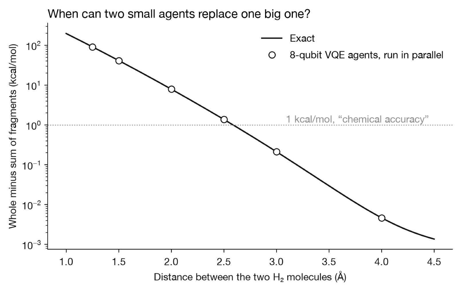
At 1.25 Å apart, the fragments are off by 91 kcal/mol. At 2 Å, 7.9. At 4 Å, 0.005. That exponential drop is nearsightedness, measured directly. Past about 2.6 Å, the two small agents are within “chemical accuracy” (1 kcal/mol) of the big one.
Small agents matter because qubit cost compounds. 8 qubits is 256 amplitudes; two separate 4-qubit fragments are 16 each. That gap grows exponentially: one 200-qubit problem is impossible to simulate classically, while twenty 10-qubit fragments are trivial. The swarm part is real, too. I ran six 8-qubit VQE agents at once, one per distance. They took 36 seconds together, versus 166 seconds one after another.
4. Binder-pocket fitting: what the fragments leave out
Builds on: layer 3. The error the swarm makes at short range is the interaction itself.
Look at layer 3’s plot again. “Whole minus the sum of the parts” has a name in drug design: binding energy.
When a drug sits in a binding pocket, that number is negative: the complex is happier together than apart. For the swarm, it’s exactly the part the fragment agents miss. So the coordinator’s job is to compute the bits where the pieces touch, and only those bits need the expensive quantum treatment. In the real version, a classical force field handles most of the protein, and quantum chemistry handles a few dozen atoms around the pocket.
My toy “pocket” is an H₂ molecule, and the “ligand” is a single proton (H⁺) approaching it from different directions:
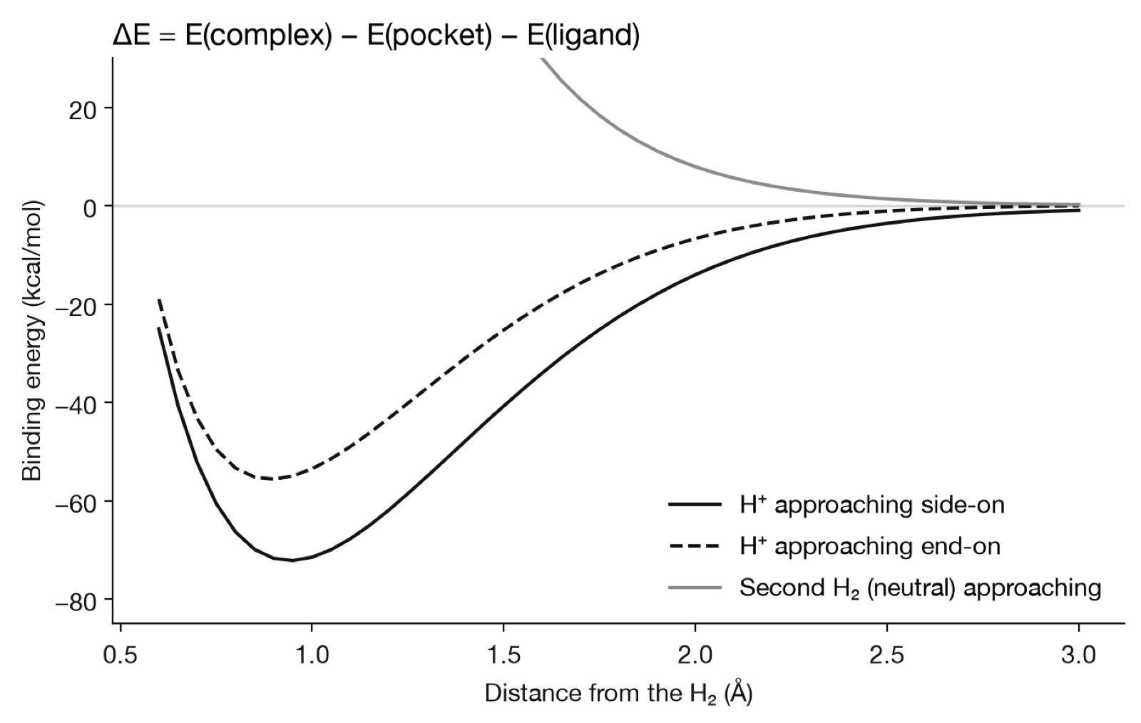
The proton binds, and it has a preferred pose. Side-on at 0.95 Å it binds by 72 kcal/mol; end-on, only 56. Side-on makes a triangle, and that’s the real shape of H₃⁺, one of the most abundant ions in the universe. A 6-qubit VQE on the best pose agreed with the exact answer. The real binding energy is closer to 100 kcal/mol. My toy undershoots because it uses the smallest possible basis and doesn’t let the H₂ bond relax.
The gray line is the more interesting failure. Two neutral H₂ molecules should attract a tiny bit through dispersion (van der Waals forces), the same weak “stickiness” that holds most drugs in their pockets. In this basis they only repel. Capturing dispersion needs a bigger basis, which means more orbitals, which means more qubits. That’s the “orders of magnitude away” the physicist told me about, made concrete.
For the binders that actually work today, like the antivenom binders I designed and the ones in the cobra paper, classical and ML tools (BindCraft, Boltz-2, Rosetta) are doing the fitting. Quantum chemistry, when it’s used at all, refines the energies at the end.
5. Quantum signals from the body: running it backwards
Builds on: layer 4. Once a binder is designed, you need to see whether it works in a living body, and you need real data to feed back into layer 2.
So far, the qubits have been computing: we know the Hamiltonian and want its energy. Flip that around. Put a qubit in the real world, let an unknown magnetic field act on it, and measure how its state changed. Now the qubit is a sensor, and the same physics makes it an extremely sensitive one.
The quantum trick is entanglement. Measure a field with n independent qubits, and your error shrinks like 1/√n, just like averaging n separate measurements. Entangle them in a GHZ state (all qubits 0 and all qubits 1 at once) and the field’s effect adds up coherently across all of them, so the error shrinks like 1/n.
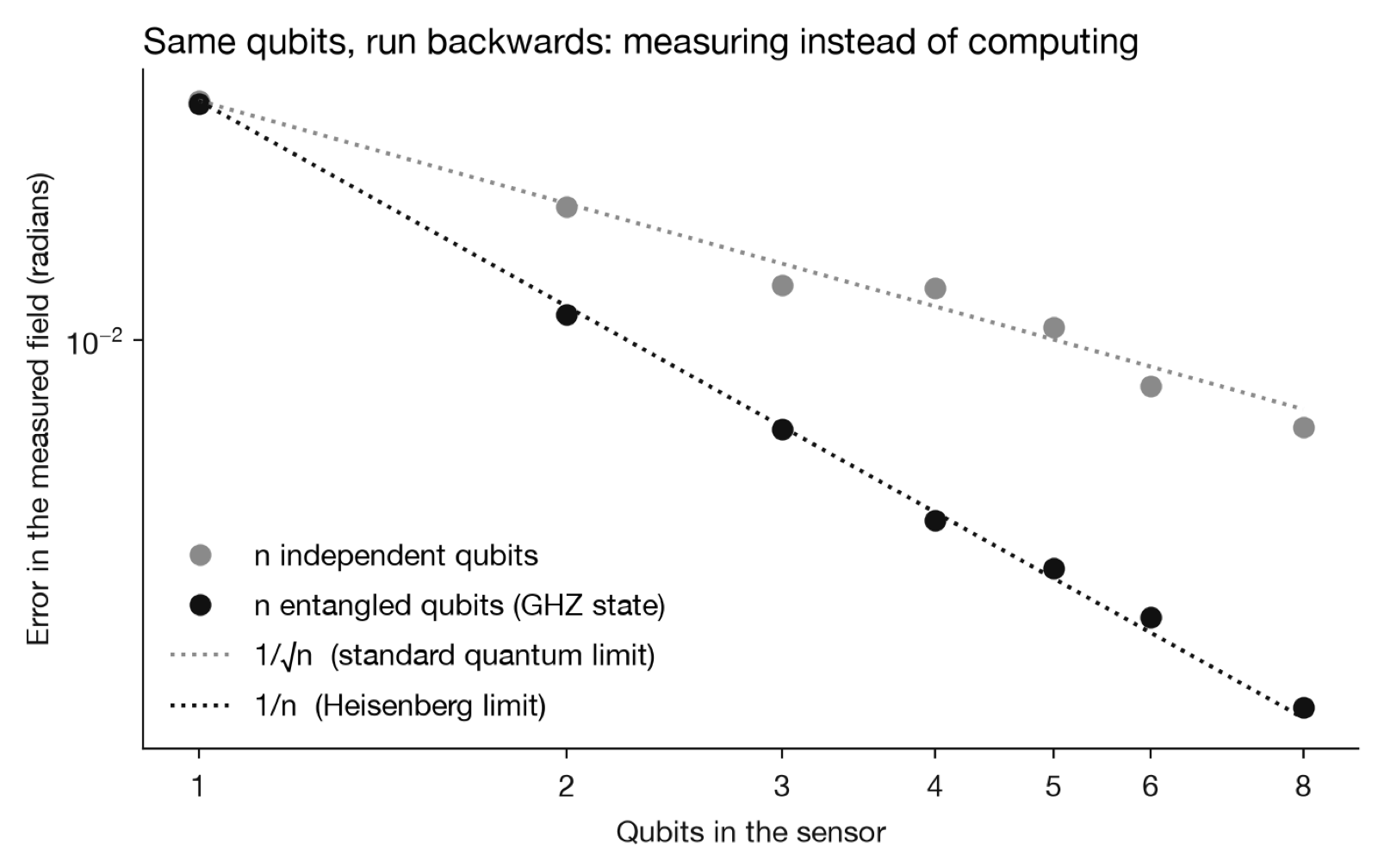
With 8 qubits and the same number of measurements, the entangled sensor is 2.6× more precise than the independent one. The gap keeps growing with n.
This is where quantum biology is real today, not in 30 years:
- Wearable brain scanners. Optically pumped magnetometers use vapor-cell atoms to pick up the brain’s magnetic fields without cryogenic cooling. In 2018, Boto et al. recorded brain activity in a person who was moving their head around.
- Diamond sensors on single neurons. Nitrogen-vacancy defects in diamond are single trapped spins. Barry et al. used them to detect the magnetic field of a single neuron’s action potential, in a living worm.
- Hyperpolarized MRI. Line up the nuclear spins of a molecule like pyruvate and its MRI signal goes up by more than 10,000×, enough to watch tumors turn pyruvate into lactate in real time. Nelson et al. ran the first human trial in prostate cancer patients in 2013.
Honest caveat: these devices use lots of unentangled spins. Entangled sensors like the one in my plot are still lab experiments. But they’re already useful, and they’re the part of this stack that closes the loop: design a binder, put it in a body, measure what it does, and feed the measurements back to layer 2.
6. Generative design: proposing new poses
Builds on: everything. Layers 1-3 score candidates, layer 4 says what a good score is, and layer 5 is how you’d eventually check the winners.
So far I’ve been scoring poses someone else picked. Generative design flips that: a model proposes poses, and the stack scores them. On a quantum computer, the generator can be a circuit. Measure n qubits and you get one n-bit string, drawn at random from a probability distribution that you shape by tuning the circuit’s angles. That’s called a Born machine.
Here, 6 qubits = 64 bitstrings = 64 poses of the proton around H₂ (8 angles × 8 distances). The pipeline:
- Layers 1 + 3: run VQE on 20 random poses, in parallel.
- Layer 2: train an ML model on those 20 and use it to score all 64.
- Turn scores into a target: better binding means more probability.
- Train the 6-qubit circuit until it generates poses at those probabilities.
- Sample 1,000 poses from it.
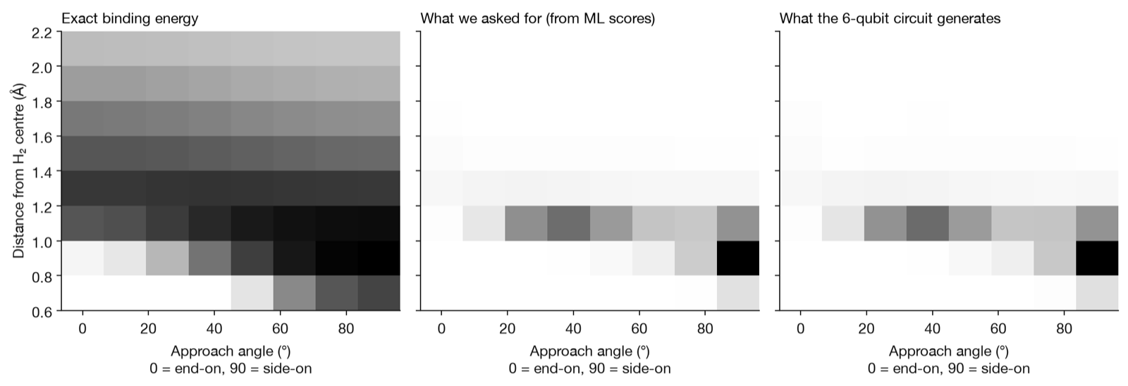
The circuit learned its target almost perfectly. The most common pose it generated (20% of samples) was side-on at 0.9 Å, which is also the true best pose.
But look at the band at 1.1 Å in the middle panel. The ML model was wrong about a band of in-between angles at 1.1 Å. At 26°, it predicted −68 kcal/mol when the truth was −54. The generator faithfully copied that mistake: 26% of its samples went to poses the ML model overrated by more than 5 kcal/mol. A generator is only as good as whatever scores it. So the real loop is: generate, send the top candidates back to the quantum computer (layer 1), add them as training labels (layer 2), retrain, and generate again.
This is roughly what the first serious attempt did. In Ghazi Vakili et al. (2025), a team used a quantum Born machine as part of a generative model for KRAS inhibitors. They made 15 molecules, and 2 looked promising in cells. The authors themselves called it a proof of principle with no sign of a real quantum advantage yet.
There’s one more thing about generation I think is underrated. My opinion is that eventually all software will be generated live, rather than loaded from disk and run by a kernel. Quantum computers already work this way, as a function of their design. The no-cloning theorem says you can’t copy an unknown quantum state, and there’s no way to save one to disk and load it later. The 64-pose distribution my circuit learned doesn’t exist anywhere as stored data. The only thing saved is the recipe: a few dozen angles. Every single sample means building the state again from scratch and measuring it once. A quantum program is always generated on the spot.
So what can you do on a quantum computer that you can’t on a classical one?
Back to the question I started with. After building all six layers, here’s my answer:
| Use | When |
|---|---|
| Measuring biology with quantum sensors (brain, neurons, metabolism) | Now, already in hospitals and labs |
| Exact energies of tiny molecules | Now, if you shrink the problem until it needs no two-qubit gates. My 4-qubit runs lost to a 1930s approximation; the 1-qubit version beat it |
| Generative models with a quantum sampler | Now, as experiments. No advantage shown yet |
| Exact energies for the hard parts of chemistry (metal active sites, bonds breaking), used as ML training labels | Someday, needs error-corrected machines with hundreds to thousands of logical qubits |
| Fragment swarms across many small quantum computers | Someday, same requirement, but it’s the most promising route to scale |
| Docking a whole binder into a whole protein on a quantum computer | Maybe someday. Classical and ML tools already do this well, and for now quantum computers are best at small, hard, accurate pieces |
So, besides breaking encryption: a quantum computer is a calculator for small, hard, very accurate pieces of chemistry, and a sensor for very small signals. It won’t design a drug by itself. But it can sit underneath an ML model, as the thing the model checks its homework against.
Using a quantum computer as the judge
That last sentence is the most realistic job for a quantum computer in drug design. At the small scale it’s already true: VQE is a classical optimizer using the quantum computer as its objective function. The optimizer proposes angles, the quantum computer returns an energy, and the optimizer adjusts.
At the big scale, it looks a lot like how LLMs get trained with human feedback. Human judgments are expensive, so you collect a few, train a cheap reward model on them, and train the main model against the reward model. Swap the humans for a quantum computer and you get:
- A cheap generator (like the Born machine in layer 6) proposes thousands of candidates.
- A cheap scorer (like layer 2’s ML model) ranks all of them. This is the reward the generator trains against.
- An expensive judge, the quantum computer, checks only a handful: the top candidates, plus the ones the scorer is least sure about. Layer 2’s uncertainty bands show exactly where to look.
- The judge’s answers become new training labels, the scorer gets retrained, and the loop goes around again.
The quantum computer can’t be the reward for every step. Each call took seconds to minutes with queueing, my runs worked out to roughly $1-2 per energy, and even my best hardware result carried about 3 kcal/mol of noise. A training run that needs millions of reward checks can’t afford that. Checking a few hundred winners is fine.
Layer 6 already showed why you need the judge. 26% of the generator’s samples went to poses the ML scorer had overrated. That’s reward hacking: the generator learned to exploit the scorer’s mistakes instead of finding good binders. Going back to the quantum computer every so often is how you catch it.
The catch is that this only pays off where a classical computer can’t produce the label. For H₂, the exact answer is free on a laptop, so here it’s a demo. The real version is a ladder of labels: a force field for millions of cheap checks, DFT for thousands of better ones, and a quantum computer for the few dozen hard pieces (metal centers, bonds breaking) where everything below it is wrong.
Code and data
Everything is on GitHub at bmwoolf/quantum-drug-design: the six layers, both rounds of hardware runs, and the raw data from Rigetti, including every circuit, task, device calibration snapshot and measurement count.